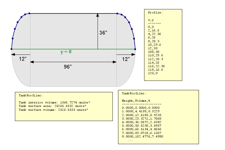
TankProfiler, like its predecessor TankCalc, analyzes and provides data for various kinds of storage tanks. For a user-provided profile, it produces content volume, tables listing incremental volume correlated with sensor height and the reverse, surface area and surface volume.

When I first wrote my storage tank analyzer TankCalc, I had the idea that most storage tanks fell into a relatively small number of categories like that shown above — central cylinders with a few easily-described kinds of end caps. But since then I have received any number of inquiries from owners of oddly-shaped tanks — tanks with something other than a simple cylindrical middle section, and with any number of peculiar end caps, caps that don't fit into simple geometric categories.

In response I have created a much more flexible program, one that, instead of making assumptions about a tank's shape, accepts a user-created dimension profile of the tank, in the form of x,y Cartesian coordinates, and models the tank on that basis.

To use TankProfiler, a user creates a plain-text file containing a dimension profile of the tank to be analyzed. Such a file might contain these x,y coordinate pairs:

0,8
30,30
130,30
160,8
            

Each x,y coordinate pair provided to TankProfiler describes the perimeter of a circle whose center lies at y coordinate zero, and the circle forms part of the desired tank profile. Expressed another way, each x,y coordinate pair describes a circle having radius y and centered at coordinate x,0. Like this:

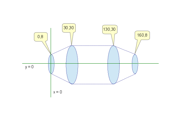
Remember that the y coordinates are radii, not diameters. With the above information, TankProfiler will model a tank that looks like this (this image is generated by TankProfiler):

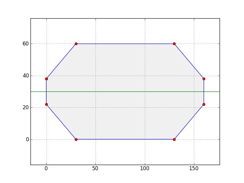
The above example is intentionally simple (nevertheless representing a tank type that the prior program TankCalc cannot manage), but TankProfiler can analyze any number of more complex tank types. Another problem tank that has come to my attention is a large storage tank with stepped sides, another type that TankCalc cannot manage (this image is also produced by TankProfiler):

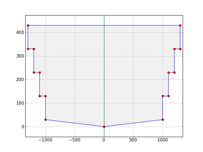
The above example uses TankProfiler's -u (upright) mode, for which the x and y coordinates are reversed. This example, whose dimensions are greatly exaggerated, turns out to be a fairly common large tank design, in which a very shallow cone (to simplify cleaning) at the bottom ascends into a series of wall sections of differing thicknesses, thickest at the bottom to bear the greater pressures, and thinnest at the top, to save construction costs. TankProfiler easily handles this complex tank type.

TankProfiler versions 1.2 and above correctly handle complex shapes with internal voids — shapes like this:

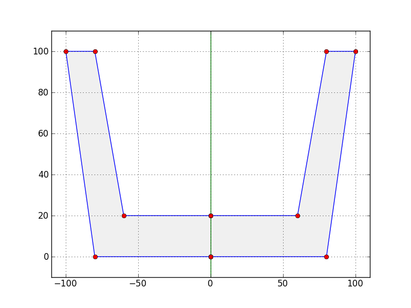
The computed volume is limited to the grayed area in the above graphic, and there is no limit to the number of volumes and voids that may be included in a complex profile. This means geometric profiles with multiple walls will be correctly analyzed. But because of this new capability, when writing tank profiles users must be sure that the profile's vectors rotate clockwise around volumes and counterclockwise around voids. Like this:

If this rule isn't followed, the profile will produce an overall negative volume, which will cause TankProfiler to exit with an error message: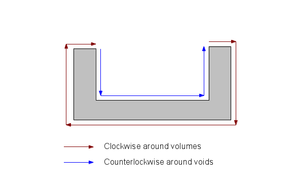

Error: volume < 0

Provided with a user-created tank profile, beyond producing a picture to assure the user that he and TankProfiler are on the same wavelength, TankProfiler can produce most of the same results that TankCalc provides:

1. A table that provides partial tank volumes for given integral sensor heights, for any given sensor step size.
2. A table that's the reverse of the above — heights for integral volumes. For reasons given below, this table requires more time to generate.
3. The tank's interior volume, surface area and (if a wall thickness is provided) surface volume.

Results (1) and (2) above can be had for two tank orientations — horizontal and vertical (upright). Result (3) can be used to compute the tank's content weight, its empty weight, and its overall weight.

NOTE: To see a typical use for TankProfiler and see how a tank profile is generated, visit the TankProfiler Case History page.

Unlike TankCalc and most of my other programs, TankProfiler is a commmand-line application without a graphical user interface (GUI). I chose this design because it allows quick changes to accommodate new requirements over time. One of the problems with this program's predecessor TankCalc is that it's locked into its GUI, which makes changes difficult. Because it is a command-line application written in Python, TankProfiler is easy to modify to meet new requireents.

TankProfiler is Copyright 2013, P. Lutus and is released under the GPL.

Here is what you need to run TankProfiler:

• The TankProfiler Python script — just right-click the link and save the script in its own directory under the name "tankprofiler.py".
• Python, available for all platforms. Choose Python 2 (TankProfiler will run on Python 3, but requires minor changes to do so).
• To support the plotting function, be sure the Python library matplotlib is installed.
• If you want to export PDF versions of the generated tables, install wkhtmltopdf.

That's it.

TankProfiler will run on any platform on which Python runs. There are some minor differences between platforms that hopefully won't cause confusion in the following instructions.

When you have installed TankProfiler in its own directory, open a command shell in that directory and type:

$ ./tankprofiler.py -h

(The '$' is the shell prompt, you don't type it.)

TankProfiler will respond with this list of options:

Usage: tankprofiler.py [options]

Options:
  -h, --help            show this help message and exit
  -a ARG, --arg=ARG     use argument to compute a single height/volume result
                        instead of a table
  -c CONV, --conv=CONV  volume conversion factor (cm続 to liters = 1000, in続 to
                        gallons = 231), default 1.0000
  -d DEC, --decimals=DEC
                        result decimal places, default 4
  -D, --draw            draw an image of the tank (and save 'tank.png')
  -f IFILE, --ifile=IFILE
                        input file path containing tank profile (x,y value
                        pairs) ('-' = stdin)
  -F OFILE, --ofile=OFILE
                        output file path (default: stdout)
  -H, --html            use HTML output format (default: CSV)
  -i INTSTEPS, --intsteps=INTSTEPS
                        integration steps (only used in horizontal mode),
                        default 1000
  -m MULT, --mult=MULT  volume multiplier for oval tanks, default 1.0000
  -n, --noprog          don't print progress chars
  -P, --pdf             use PDF output format (default: CSV)
  -p, --plot            plot coordinate points in graphic image
  -r, --rev             create volume -> height table (default height ->
                        volume) — slower.
  -s STEP, --step=STEP  table increment size, default 1.0000
  -S SOFFSET, --soff=SOFFSET
                        sensor offset value, default 0.0000
  -t TITLE, --title=TITLE
                        HTML/pdf page title (default none)
  -u, --upright         upright (vertical) tank mode (x and y reversed)
  -v, --version         program version and additional information
  -V VOFFSET, --voff=VOFFSET
                        volume offset value, default 0.0000
  -w WALL, --wall=WALL  tank wall thickness, default 0.0000
  -x, --extra           compute full volume, surface area, surface volume (if
                        wall thickness provided)
            

Here are detailed explanations for the options:

-h, --help            show this help message and exit
          

The option list is also displayed if no command options are provided.

-a ARG, --arg=ARG     use argument to compute a single height/volume result
                      instead of a table
          

Normally TankProfiler generates a table of results, for the entire height and volume of the tank. If this entry is made, TankProfiler instead creates a single result for the provided argument.

-c CONV, --conv=CONV  volume conversion factor (cm続 to liters = 1000, in続 to
                      gallons = 231), default 1.0000
          

This is a convenient way to convert volume results from cubic units into a more useful volume unit like gallons or liters. Any conversion factor may be entered. Remember that cubic units are divided by this factor to produce the displayed result.

-d DEC, --decimals=DEC
                      result decimal places, default 4
          

For reasons explained below, the default horizontal mode uses numerical integration and is therefore approximate (the upright (vertical) mode is exact). Because of this, remember when choosing displayed decimal places that not all displayed digits are necessarily meaningful. One way to increase numerical accuracy in the horizontal mode is to increase the number of integration steps (option -i below). This increases accuracy at the expense of runtime.

-D, --draw            draw an image of the tank (and save 'tank.png')
          

This option will draw an image of the profiled tank if your system's Python installation has the matplotlib library installed. Some of the images in this article were generated using this option.

-f IFILE, --ifile=IFILE
                      input file path containing tank profile (x,y value
                      pairs) ('-' = stdin)
          

This option provides TankProfiler with a set of Cartesian x,y data pairs describing the tank as explained in the previous section. A typical entry might be:

$ ./tankprofiler.py -f myprofile.txt

The provided file should be plain text, but beyond that, the only formatting requirement is that numerical values for x and y follow each other in sequence, separated by whitespace or any other non-numeric characters.

Another option is to specify '-' as the "file name", which tells TankProfiler to read the standard input for its profile data. Here is an example:

$ echo "0 8 30 30 130 30 160 8" | ./tankprofiler.py -f -

-F OFILE, --ofile=OFILE
                      output file path (default: stdout)
          

This option allows entry of a file name for the output data. If no entry is made, the output appears on the standard output. Here are three ways to direct the program's output:

• $ ./tankprofiler.py -f myprofile.txt [output appears on the console]
• $ ./tankprofiler.py -f myprofile.txt > output.txt
• $ ./tankprofiler.py -f myprofile.txt -F output.txt

When using the -H (HTML) and -P (PDF) output options described below, one may (should) specify a file name with an appropriate suffix.

-H, --html            use HTML output format (default: CSV)
          

The default TankProfiler output format is CSV — simple comma-separated values, suitable for entering into a database or spreadsheet program. This option instead creates an HTML-formatted page containing a table of results that looks more or less like this:

Height	Volume	%
0.0000	0.0000	0.0000
10.0000	33358.4354	9.8318
20.0000	94520.7965	27.8582
30.0000	169645.9962	50.0000
40.0000	244771.1959	72.1418
50.0000	305933.5570	90.1682
60.0000	339291.9925	100.0000

-i INTSTEPS, --intsteps=INTSTEPS
                      integration steps (only used in horizontal mode),
                      default 1000
          

This option is used to increase the accuracy of the numerical integrator used in the TankProfiler default horizontal mode. For most applications the default number of integration steps is more than adequate. Increasing the number of integration steps increases runtime.

-m MULT, --mult=MULT  volume multiplier for oval tanks, default 1.0000
          

This is an easy way to acommodate tanks that have an oval cross-section. The entry represents the ratio of tank width to height, like this:

As an example, for a tank that is 36 inches in height and 48 inches in width, the provided profile would describe a cylindrical tank with an 18-inch radius (i.e. 36-inch diameter), and the -m option entry would be (48/36) 1.3333... With this option, all the volume values are adjusted to take the tank's width into account, while the height values are correct for the tank's overall height.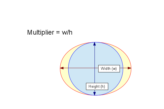

-n, --noprog          don't print progress chars
          

Normally, during lengthy table generation, progress dots are printed to the console. This option suppresses the dots.

-P, --pdf             use PDF output format (default: CSV)
          

As with the HTML option described above, instead of the default CSV output format, this option creates a PDF version of the generated table. This option requires that the wkhtmltopdf program be installed on your system.

-p, --plot            plot coordinate points in graphic image
          

This option plots terminating coordinate points for each line of the graphic image (as in most examples on this page)

-r, --rev             create volume -> height table (default height ->
                      volume) — slower.
          

By default, TankProfiler creates an incremental table that correlates integral sensor heights with partial tank volumes. This option reverses the relationship and produces a table that correlates integral volumes with sensor heights. To do this, and because of the complexity of the required calculations, TankProfiler uses a root finder method. Root finders are easy to write but run slowly (they typically require eight times the processor time to arrive at a result).

-s STEP, --step=STEP  table increment size, default 1.0000
          

This option accepts a table step size, either in height units or (for the -r reverse mode) volume units. This allows the user to choose the desired table resolution.

-S SOFFSET, --soff=SOFFSET
                      sensor offset value, default 0.0000
          

TankProfiler normally profiles the entire tank, from zero height to full height. This option accommodates any physical or other limitations that require the height scale to be offset by a fixed amount. Also see option -V below.

-t TITLE, --title=TITLE
                      HTML/pdf page title (default none)
          

This option accepts a title to be included with the -H HTML or -P PDF output options. Remember to encliose multi-word titles in quotes:

$ ./tankprofiler.py -f myprofile.txt -H -t "This is my table"

-u, --upright         upright (vertical) tank mode (x and y reversed)
          

This option analyzes the tank in an upright orientation, as shown in the prior section — the tank's x and y coordinates are reversed. In the default horizontal mode, to produce partial volumes that correspond to sensor heights, an approximate numerical integration method must be used (described below). But in the upright mode, no numerical methods are required and the results are exact (at least as exact as the provided profile data). Because there is no numerical integration, the upright mode produces its results much faster.

-v, --version         program version and additional information
          

This option prints the program version, a copyright notice, and provides an URL for the TankProfile home page.

-V VOFFSET, --voff=VOFFSET
                      volume offset value, default 0.0000
          

TankProfiler normally profiles the entire tank, from zero volume to full volume. This option accommodates any physical or other limitations that require the volume scale to be offset by a fixed amount. Also see option -S above.

-w WALL, --wall=WALL  tank wall thickness, default 0.0000
          

This option accepts wall thickness information in the same units as the tank's dimensions, to allow a tank's surface volume to be computed. See -x below.

-x, --extra           compute full volume, surface area, surface volume (if
                      wall thickness provided)
          

This option computes some extra values that are useful in a complete tank analysis, i.e. the full analytical volume (not an approximation), the tank's surface area in the input units squared, and the surface volume in the input units cubed if a wall thickness has been provided (see option -w above).

In essence, TankProfiler is a convenient wrapper around mathematical methods that generate its results. This section describes the equations and algorithms that produce those results.

The basic purpose of TankProfiler and its predecessor TankCalc is to correlate the position of a content-height sensor with the tank's partial content volume. For an upright cylindrical tank, such a correlation is trivial:

(1) Volume $ \displaystyle v = \pi r^2 y$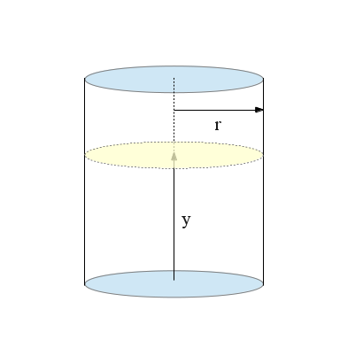

Where y = sensor height. But most tanks have a different shape or orientation, which makes the math more complicated. The next case beyond an upright cylinder, in terms of increasing complexity, is a horizontal cylinder:

(2) $ \displaystyle y' = \frac{y}{r} - 1$

(Note the variable ranges: 0 ≤ y ≤ 2r and -1 ≤ y' ≤ 1)

(3) $ \displaystyle v = r^2 l \sqrt{1-y'^2} y' \cos^{-1}(-y')$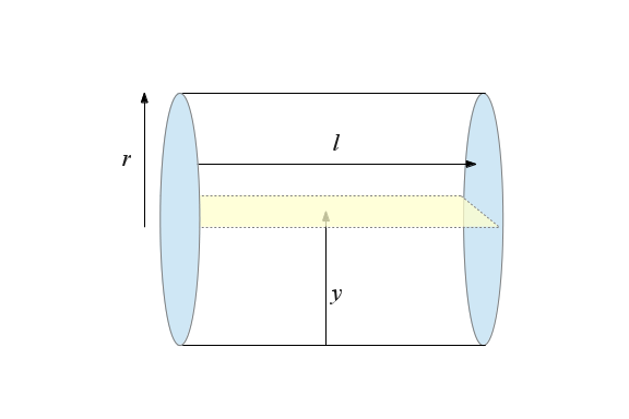

Volume in Horizontal Mode

A version of the above equation has multiple applications, so here it is in a simpler, more universal form that provides a partial circle area a for a given argument y within a unit circle:

(4) $ \displaystyle a = \sqrt{1-y^2} y \ \cos^{-1}(-y), -1 \leq y \leq 1$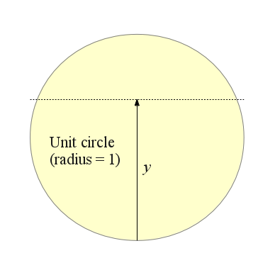

The above equation is the key to the numerical integration method used in TankProfiler to compute frustum partial volumes in the horizontal mode. For tank sections that are in essence conical frustums, the numerical method uses this general scheme (for simplicity some details are left out):

(5) $ \displaystyle y' = \frac{y}{r}-1$

(6) $ \displaystyle v = \sum_{i = 1}^n{ r^2 \sqrt{1-y'^2}} y' \ \cos^{-1}(-y') \frac{x_b-x_a}{n}$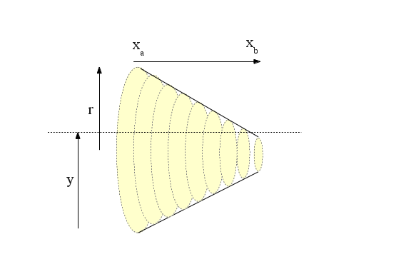

The number n of summed disc results is governed by the TankProfiler -i value (default 1000), which is more than adequate for normal purposes.

Volume in Upright (vertical) Mode

For the TankProfiler upright mode, closed-form equations are used and there is no numerical computation, so the results are closed-form and as accurate as the user-supplied profile data. All tank sections that are not bisected by the sensor height y value are modeled as conical frustums using these area and volume equations (source):

(7) $ \displaystyle s = \sqrt{(r_a-r_b)^2 + h^2}$

(8) $ \displaystyle a = \pi (r_a+r_b) s $

(9) $ \displaystyle a = \pi (r_a+r_b) \sqrt{(r_a-r_b)^2 + h^2}$

(10) $ \displaystyle v = \frac{1}{3} \pi h (r_a^2 + r_a r_b + r_b^2)$

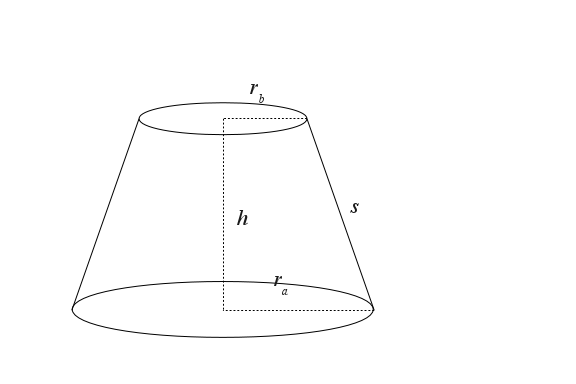
It's important to add that the above equations, meant to compute volumes and surface areas for conical frustums, are valid for the limiting cases where h = 0 (disk/washer) and r_a = r_b (cylinder).

While computing values for the above closed-form frustums as part of a complex tank, TankProfiler eventually gets to a frustum that's bisected by the y value (the sensor height). At that point equations written by the author are used to correlate sensor height y and the partial volume of the bisected frustum:

(11) volume v for sensor height y: $ \displaystyle v = \frac{{\left(3 \, h^{2} r_{a}^{2} y + {\left(r_{a}^{2} - 2 \, r_{a} r_{b} + r_{b}^{2}\right)} y^{3} - 3 \, {\left(h r_{a}^{2} - h r_{a} r_{b}\right)} y^{2}\right)} \pi}{3 \, h^{2}}$

(12) sensor height y for volume v: $ \displaystyle y = \frac{h r_{a}}{r_{a} - r_{b}} - \frac{\left(\frac{{\left(\pi h r_{a}^{3} - 3 \, {\left(r_{a} - r_{b}\right)} v\right)} h^{2}}{\pi}\right)^{\frac{1}{3}}}{r_{a} - r_{b}}$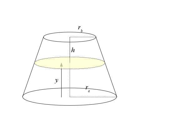

When computing surface area and surface volume, the same method is used in both the horizontal and upright modes. This means that, regardless of the selected mode, the surface computations are not approximate, but are as accurate as the provided data.

• Conical Frustum (MathWorld)
• TankCalc
• Storage Tank Profiling
• TankProfiler Case History

• 2013-01-27 Version 1.4. Set 1:1 aspect ratio for graphic output, made plotted points an option.
• 2013-01-25 Version 1.3. Refactored output formatter class for future use as a separate executable.
• 2013-01-03 Version 1.2. Recoded volume routines to accommodate complex shapes with voids.
• 2012-12-24 Version 1.1. Tuned the plotting function for better appearance.
• 2012-12-20 Version 1.0. Initial Public Release.