

 Share This Page
| Home | | Mathematics | | * Sage | |  |  |  Share This Page Share This Page |
Exploring the Frequency Domain
— P. Lutus — Message Page — Copyright © 2009, P. Lutus(double-click any word to see its definition)
To navigate this multi-page article:Use the drop-down lists and arrow icons located at the top and bottom of each page.
Click here to download the
Sage worksheet used in preparing this article.
If you have access to Sage and would like to interact with this article's content, either download the worksheet linked above or copy the contents of this cell into your running Sage session:
#auto
reset()
forget()
# special equation rendering
def render(x,name = "temp.png",size = "normal"):
    if(type(x) != type("")): x = latex(x)
    latex.eval("\\" + size + " $" + x + "$",{},"",name)

# magnitude of 2-component cartesian vector
def mag(x):
    return sqrt(x[0]^2+x[1]^2)

var('a, b, c, d, f, g, m, q, t, x, y')

# time-domain function plot
def time_plot_funct(funct,nl,w=0.25,color='#006000',labels=('Time','Amplitude')):
    n = 500
    list = [[t*w/n,funct(t*w/n,nl)] for t in range(n)]
    return list_plot(list,rgbcolor=color,axes_labels=labels,plotjoined=True)

# time-domain FFT array plot
def time_plot_fft(fftobj,freq,line_color='#006000',labels=('Time','Amplitude')):
    lfft = len(fftobj)
    data = [[x*2*freq/lfft,fftobj[x][0]] for x in range(lfft/2)]
    return list_plot(data,plotjoined=True,rgbcolor=line_color,axes_labels=labels)

# frequency domain plot
def fft_plot(fftobj,line_color='#006000',labels=('Frequency','Amplitude')):
    size = len(fftobj)
    dt = 1.0/size
    list = map(lambda x:(mag(x))*dt,fftobj[:size/2])
    return list_plot(list,rgbcolor=line_color,plotjoined=True,axes_labels=labels)
Some of the earlier articles in this set are helpful in setting the stage for this one, in particular Tuned Circuits because of its discussion of complex numbers.
Many mathematical disciplines, though fascinating, have little practical utility, while others are the reverse (useful but not interesting). Because of innate complexity or computational workload, some disciplines had few practical applications until people began to apply computers to mathematical problems. Fourier methods fall into the latter category — until recently, it was an esoteric field with much theoretical substance but few tangible applications.
In mathematics and at present, the computer is properly seen as an inferior partner, freeing people to view mathematical ideas from a higher vantage point while churning out pedestrian results. (Someday computers may generate their own mathematical ideas, but we aren't there yet.) With respect to the present topic, the computer's ability to produce practical results has turned an esoteric mathematical field into a practical one that is central to much of modern technology — applications for Fourier methods abound in nearly every part of modern science and technology:
- Efficient data compression in graphics, video and television
- Analysis of general periodic data
- Signal detection and recovery in noisy environments
- Fourier Deconvolution in seismology and optics
- Ocean tide predictions
And many others. The basic idea of the Fourier Transform is that a periodic function in the time domain has an equivalent form in the frequency domain, and further, that these forms are interchangeable:
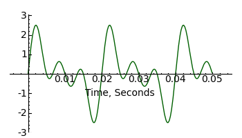

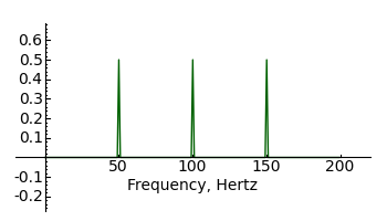
The first thing to understand about Fourier methods is that the frequency representation of a periodic waveform may represent a much smaller amount of information than the time representation. In the above example the right-hand graph contains only three data points, but those points are adequate to fully reconstruct the time-domain wave at the left. This greatly simplifies the description and reconstruction of periodic waves.
This economy of description is one reason Fourier methods are so widely used to compress data streams to a small fraction of their original size, and is the primary reason old-style analog television has been replaced by the newer, much more efficient digital methods.
The second thing to understand is that Fourier methods may be used to recover signals apparently lost in noise:
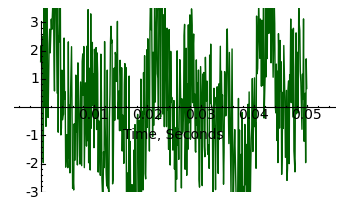

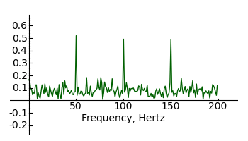
The above graphs show how easily periodic signals can be made to pop out of background noise. More sophisticated Fourier methods are used to extract very weak signals from distant spacecraft and cosmological sources in the presence of high natural noise levels.
Sage is able to perform many kinds of Fourier operations, including symbolic transforms and the numerical Fast Fourier Transform to be described later. Before we explore these applications, let's look at the mathematical underpinnings.
Using somewhat simplified notation, the Fourier Transform of a time-domain function f(x), for real numbers x and y, looks like this:
(1)
And the inverse Fourier Transform looks like this:
(2)Where:
- f(x) = a time-domain function
- f(y) = a frequency-domain function
- x = an argument with units of time
- y = an argument with units of frequency
- e = the base of natural logarithms
- i = the imaginary unit (i2 = -1)
Euler's Formula
At first glance it may seem counterintuitive that the simple exponentiation shown above (e±2πixy) can produce a transformation between the time and frequency domains. But the expression at the heart of the Fourier integral makes this possible. Called Euler's Formula, it has an interesting property:(3)
The relationship expressed by Euler's Equation turns out to be ideal for representing time-varying waves in a compact frequency-domain form and the reverse. We can use Sage to graph this key property of Euler's Equation:
lbl = text("$e^{2\pi i \\theta} = cos \, 2\pi\\theta  + i \, sin \, 2\pi\\theta $"
,(1,1.2),fontsize=14,rgbcolor='black')
rp = plot(lambda x:N(e^(2*pi*i*x)).real(),x,0,2,rgbcolor='#006000')
ip = plot(lambda x:N(e^(2*pi*i*x)).imag(),x,0,2)
show(rp+ip+lbl,figsize=(4,3))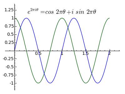
The green trace represents the real part and the blue trace represents the imaginary part of the Euler's Equation result. (Some of the complexity in the above worksheet cell represents workarounds for bugs in the present version of Sage (4.1.2)).
The above represents the foundation on which all Fourier methods are built. Next, we turn to a practical method for analyzing real-world data sources that aren't continuous.
The Discrete Fourier Transform (DFT), derived from the above method, represents a way to process discontinuous data, for example data sampled at regular time intervals from a source such as a radio receiver. Because the data take the form of a set of discrete samples, the analysis method changes:
(4)
And the inverse DFT:
(5)Where:
- xn = a complex time-domain data set
- Xk = a complex frequency-domain data set
- N = the size of the data sets (which are assumed to be equal)
It can be seen that the continuous integration of the Fourier Transform (equations (1) and (2) above) has been replaced by a summation of discrete terms in the corresponding DFT (equations (4) and (5)). The notation used in the above DFT equations is a bit nonstandard and bears explanation — for each of the DFT equations one sees two indices: n and k. A careful look at the equations reveals that there are two nested loops, both with size determined by N, the size of the data sets, so it's reasonable to assume the DFT becomes very slow for large data sets — and this is true (a DFT over N data points requires O(N2) operations).
Nyquist-Shannon Sampling Theorem
One important property of the DFT merits special attention. According to the Nyquist–Shannon sampling theorem, to properly analyze a band of frequencies extending up to some upper limit of N Hertz, one must gather data at time intervals of 1/(2N) — for example, a maximum frequency of 100 Hz would require a minimum sampling rate of 1/200 second. Why this is true is easier to show than to tell:
ff(f,t) = sin(2*pi*f*t)
f = 5
@interact
def _(n = (5..20)):
    list = [ff(f,t/(2*n)) for t in range(0,n)]
    show(list_plot(list,plotjoined=True),figsize=(4,3))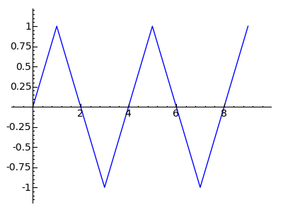
The above plot is the result for a 1/(2N) sampling rate — just enough to analyze the data. By the way — those readers who are not pasting these examples into Sage are missing out — the "@interact" feature shown above produces an interactive user control (not shown here) that changes the sampling rate and redraws the graphic.
Fast Fourier Transform
Because of the slowness of the classical DFT, a method called the Fast Fourier Transform (FFT) has been devised, which improves the speed to O(N log N) operations (an improvement roughly proportional to N/log(N)). Many people think the FFT dates back only to the 1960s and the Cooley-Tukey algorithm, but various forms of, and steps toward, the FFT date back to Carl Friedrich Gauss (1777-1855), who used an early version of the FFT to convert asteroid sightings into orbital predictions.
Most modern DFT computations are actually performed as FFTs behind the scenes, and because the FFT outcome is identical to a DFT with the sole difference that it's much faster, I won't dwell on the FFT except to say that it's the method used for nearly all Fourier operations on real-world, incremental data sets.
Recovering Spectral Lines
It turns out that Fourier methods can be used to create or analyze any imaginable periodic waveform. To be more specific, any waveform can be constructed out of a set of frequency-domain data points. Conversely, an unknown waveform can be converted into a compact set of unique spectral lines for analysis. Here's an example — let's use Sage to create and analyze a complex waveform. Copy this cell's contents into Sage:
# declare constants
epsilon = 1e-12
samples = 25

# define a waveform-generating function (wgf)
wgf(t) = 12*sin(t*3) + 11*sin(t*4) + 10*sin(t*5) + 9*sin(t*6)

# display the time-domain waveform for the wgf
show(time_plot_funct(wgf,0,10),figsize=(4,3))

# create a Fast Fourier Transform object
# and populate it with wgf data
fft = FFT(samples)
for t in range(samples):
    fft[t] = wgf(2*pi*t/samples)

# convert to frequency domain
fft.forward_transform()

# locate and print spectral lines
for f in range(samples/2):
    v = 2*mag(fft[f])/samples
    if(v > epsilon):
        print "Frequency: %3.0f, Amplitude: %3.0f" % (f,v)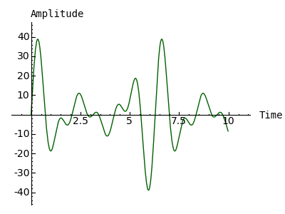
Frequency:   3, Amplitude:  12
Frequency:   4, Amplitude:  11
Frequency:   5, Amplitude:  10
Frequency:   6, Amplitude:   9
An Unknown Spectrum
The above example is meant to show the steps in the analysis process — construct a waveform, then analyze its spectrum. But we knew what the result would be, since we wrote the function to be analyzed. Let's try a more challenging example by creating a waveform whose spectrum is unknown.
# declare constants epsilon = .05 samples = 1000 # define a waveform-generating function (wgf) def wgf(t,nl): return sgn(N(cos(2*pi*t))) # display the time-domain waveform for the wgf show(time_plot_funct(wgf,0,2),figsize=(4,3)) # create a Fast Fourier Transform object # and populate it with wgf data fft = FFT(samples) for t in range(samples): fft[t] = wgf(t/samples,0) # convert to frequency domain fft.forward_transform() # locate and print spectral lines for f in range(samples/2): v = mag(fft[f])/(samples*2/pi) if(v > epsilon): print "Frequency: %3.0f, Amplitude: %.4f" % (f,v)Okay, based on the plot, it seems we've created a square wave — a wave that moves from -1 to 1 abruptly, and spends an equal amount of time at -1 and 1 (e.g. has an average value of zero). Now look at the list of spectral lines — there are lines located at frequencies of 1, 3, 5, 7 ... okay, it seems there is a spectral line at each of the odd multiples of the base frequency (such multiples of a base frequency are called "harmonics"). And the amplitudes are 1 for the first harmonic, 0.3333 for the third, 0.2000 for the fifth, 0.1428 for the seventh ... hmm. Well, 0.3333 is a pretty good approximation of 1/3, 0.2000 seems like 1/5, and 0.1428 might be ... umm ... let's use Sage to check that last one: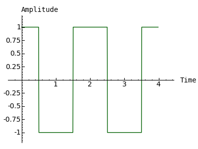
Frequency: 1, Amplitude: 1.0000 Frequency: 3, Amplitude: 0.3333 Frequency: 5, Amplitude: 0.2000 Frequency: 7, Amplitude: 0.1428 Frequency: 9, Amplitude: 0.1111 Frequency: 11, Amplitude: 0.0909 Frequency: 13, Amplitude: 0.0769 Frequency: 15, Amplitude: 0.0666 Frequency: 17, Amplitude: 0.0588 Frequency: 19, Amplitude: 0.05261/0.1428 [shift-Enter]7.00280112044818So 0.1428 is about 1/7. But we can get Sage to perform this 1/x operation for all the harmonics. Let's rewrite just one line of the above Sage cell, the one that prints the numerical results. Copy the content below and use it to replace that one line, then run the cell again (remember to indent the new content just like the old):
print "Frequency: %3.0f, Amplitude: 1/%.0f" % (f,1/v)Frequency: 1, Amplitude: 1/1 Frequency: 3, Amplitude: 1/3 Frequency: 5, Amplitude: 1/5 Frequency: 7, Amplitude: 1/7 Frequency: 9, Amplitude: 1/9 Frequency: 11, Amplitude: 1/11 Frequency: 13, Amplitude: 1/13 Frequency: 15, Amplitude: 1/15 Frequency: 17, Amplitude: 1/17 Frequency: 19, Amplitude: 1/19Square Wave Theory
Okay, we now have a theory about square waves — it seems they are composed of odd-numbered harmonics (multiples of the base frequency), each with an amplitude that is the reciprocal of its harmonic number. That seems simple enough, but how can we test this theory? In the above example, we wrote a simple function that created a square wave in the time domain, then we used a Fast Fourier Transform to convert the result into the frequency domain, then by examining the spectral lines we developed a theory about what a square wave's spectrum is.
At this point, remember that the Fourier Transform and its inverse are reciprocal operations — one operation is the exact opposite of the other. On that basis, maybe we can turn the above process around — maybe we can start in the frequency domain, write a function that creates spectral lines, transform them to the time domain, and see what the time-domain waves look like? Let's try that:
# declare constants
samples = 5000

@interact
def _(frequency = (1..8),harmonics = (1..64)):
    # create a Fast Fourier Transform object
    fft = FFT(samples)

    # populate the FFT object with spectral data
    fd2 = frequency*2.0
    for n in range(harmonics):
        a = fd2*(1+n*2)
        b = -fd2*4/(a*pi)
        fft[a] = (0,b)

    # convert from frequency domain to time domain
    fft.backward_transform()

    # display the result
    show(time_plot_fft(fft,1),ymin=-1.3,ymax=1.3)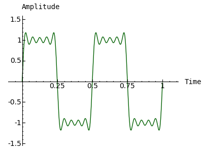
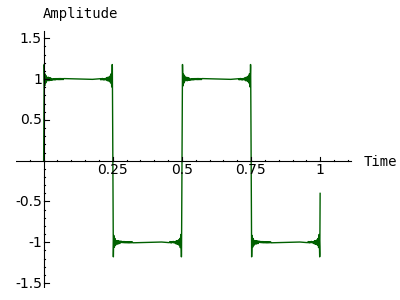
That looks promising. Again, those of my readers who are not copying these examples into Sage are really missing out — the above is actually an interactive example with two sliders, for frequency and for the number of generated harmonic lines. As the number of generated harmonic lines increases, the plot eventually looks like this (64 harmonics):
Formal Definition
By experimenting with the above Sage code I found that (1) a multiplication by 4/π normalized the result (e.g. made the steady-state values equal to -1 and 1), (2) odd-numbered spectral lines are all we need and (3) each spectral line's amplitude is the reciprocal of its harmonic number. I also concluded that an ideal square wave would have an infinity of spectral lines. This experiment leads to a formal definition of a square wave in the time domain:
(6)Where:
- y = the wave's amplitude as a function of time
- t = time, seconds
- f = frequency, Hertz
Readers may wonder why the above square wave plot, created using a frequency-domain to time-domain conversion, doesn't have clean transitions between -1 and 1, instead each transition has noticeable artifacts. It turns out these artifacts are caused by the limited resolution of the generating system — if a larger Fourier transform array is used, and if more harmonics are generated, this effect declines. Here is a plot using an array size of 500,000 data points and 16,384 generated harmonics:
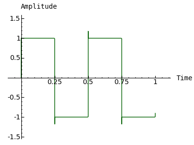
But the irony of this apparently clean plot is that the artifacts seen earlier haven't gone away — instead, because of the greatly increased resolution, they're just too narrow for the plotting code to resolve and draw.
Fourier methods are a powerful and fascinating branch of mathematics, with many practical applications — they're well worth studying. But I want to emphasize something about the examples on this page — much effort is expended to get certain results that are sometimes thwarted by various computer limitations, and in some cases we make an educated guess about the identity of a function or the meaning of a result. I want to emphasize that this activity represents a limited kind of mathematics, with much breadth but little depth. (But if the reader comes away with an understanding of Fourier methods, then this page's purpose is served.)
I mentioned earlier that computers are ideally a sort of assistant, not a full partner in mathematical activities — able to produce results a human cannot, but needing a human's guidance about which problems to tackle and how to tackle them. As we ascend through the levels of mathematics, moving from simple operations to higher levels of abstraction, the relationship between human and computer reverses. A computer can produce some kinds of low-level results almost instantly — much faster than the most adept human — but beyond a certain conceptual depth, for its own protection the computer needs to head back to the shallow end of the pool.
As time passes and as mathematical software improves, the competence line between computer and human (the line below which the computer can produce better results) continues to rise. But by freeing humans from tedious, uncreative kinds of calculation, this trend frees humans to explore mathematical territories previously too difficult to approach. This page's topic is an example — Fourier methods now see much wider application, and are much better understood, than before computer mathematics.
This may sound overly optimistic, but I anticipate a nice outcome for computers in mathematics — people will progressively understand more mathematics and be more comfortable with mathematical methods and ideas. I think this will happen because we no longer have to produce low-level results by hand — that liberation motivates people who might otherwise miss the entire mathematical adventure.
There are a number of additional Fourier-method resources here at arachnoid.com, for environments other than Sage:
"Exploring Mathematics with Sage" by Paul Lutus is licensed under a
Creative Commons Attribution-Noncommercial-Share Alike 3.0 United States License.
| Home | | Mathematics | | * Sage | |  |  |  Share This Page Share This Page |