
 Share This Page
| Home | | Mathematics | |  |  |  Share This Page Share This Page |
Copyright © 2013, Paul Lutus — Message Page
Version 1.3 (06.17.2014)
(double-click any word to see its definition)
Click here to download this article in PDF form
NOTE: This article covers discrete-value statistical analysis. For continuous distributions, my Introduction To Statistics article is probably a better choice.

Everyday life is filled with possible applications for probability theory, but few are exploited. The reason? People tend to be unfamiliar with probability ideas, and probability results are rather inaccessible. By including interactive calculators that actually work, and an in-depth mathematical exposition, this article plans to remedy both problems.
As to this article having calculators that actually work, while preparing this piece I surveyed online statistics and probability calculators, and discovered that most of them fail when presented with anything but small numbers, a crippling limitation. The reason is usually naive algorithm design, an issue I explore below.
This article is partitioned into two themes: applications of probability theory, followed by an exposition of the mathematical methods and algorithm design. If you see too few equations for your taste in the first section, don't worry — just read on.
Statistics and probability are interesting subjects with many practical applications, well worth studying. It's my hope that this article will inspire curiosity about the topics and the computation methods as well.
Let's start with one of the simpler applications of probability — the idea of a combination, generally meaning n objects taken k at a time, in any order.
Here's an example of a question we can answer with a combination — how many unique five-card hands can be dealt from a 52-card deck? Let's see — select "Combination" below and press "Compute":
That's a lot of hands of cards. Remember that, in the meaning of combination, and in real card play, the order of the cards doesn't matter — the set {King, Queen, Jack, 9, 8} is equivalent to {King, 8, Queen, Jack, 9}.
Think of all the ways that a combination result could be useful. Here's an example — in a class of 30 students, how many four-person cliques can be formed? Above, enter n = 30, k = 4, then press "Compute". Wow — 27,405 is a lot of cliques. One wonders how anyone has time to study.
A related calculation is called a permutation, much like the combination idea, but one in which order does matter. Here's an example — a locksmith must open a safe having a four-digit code (for a reason that should be obvious, I avoid use of the word combination), each number between 0 and 9, so at first glance he assumes the total number of unique codes is (10 x 10 x 10 x 10) = 10,000 (or 104). The locksmith knows he can test a code in five seconds, so he computes that, in the worst case, the job will require 50,000 seconds or about 13 hours and 53 minutes.
But being a seasoned professional, the locksmith knows about this particular model safe that digit repetitions aren't allowed by the mechanism, i.e. 4321 is a valid code but 4331 isn't. So he computes the worst-case time using a permutation, a result in which the order of the digits matters and (in the most common permutation form) repetitions aren't allowed. In the above calculator, enter n = 10, k = 4, choose permutations, and compute a result of 5,040 possible codes that meet these requirements. On that basis, at five seconds per code, the locksmith knows the job will require 25,200 seconds or seven hours.
Beyond providing relatively simple results on their own, when combined with more mathematical elements the above combination and permutation functions serve as components in more sophisticated binomial probability results, our next topic.
Binomial probability concerns itself with measuring the probability of outcomes of what are known as Bernoulli Trials, trials that are independent of each other and that are binary — with two possible outcomes.
The simplest binomial probability application is to use the probability mass function (hereafter PMF) to determine an outcome expressed this way:
What does "exact" mean above? It means the problem statement includes an exact outcome expectation expressed as a positive integer — not "up to k successes" or "k or more successes" — that form will be addressed later.
Here's a sample problem: in 100 tosses of a fair coin, each having a probability of coming up heads (call that "success") of 1/2 (0.5), what is the probability that 50 of those tosses will be successful? (I chose this example to make a point — about the meaning of exact.) Press "Compute" below:
The reader's initial reaction to this result may be that it contradicts common sense — why is the probability of 50 successes out of 100 tosses of a fair coin not equal to 1/2? The answer is that the probability mass function doesn't compute all possible experimental outcomes from zero to k, it only computes the outcome for the exact entered k value.
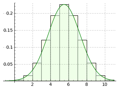
Think about this. Because of the probabilistic nature of the coin-toss experiment, in a given test the result might be less than, or greater than, 50 successes (see Figure 1 for an example distribution of outcomes). As it turns out, the probability for an outcome less than or greater than 50 successes is much greater than for exactly 50 successes, and in this case, outcomes other than 50 happen in over 92% of the tests.
What if we increase the number of tests? Let's try 1000 tests and an expected result of 500 successes (enter n = 1000, k = 500, press "Compute"). The outcome may be surprising — at first glance, one may think that increasing the number of tests should have increased the number of successes. But the criterion isn't successful outcomes, it's the number of outcomes that exactly matched k, and the exact integer value 500 is a smaller percentage of 1000 than 50 is of 100.
Here's another example problem, a bit more difficult to think through. A certain disease kills 62% of those who contract it. Of a randomly selected group of 12 patients with the disease, what is the probability that 5 will survive? Let's convert this word problem into suitable entries for the above calculator:
In the above calculator, enter n = 12, k = 5, p = 0.38, press "Compute". The result means there is about a 22% probability that exactly five patients will survive — with emphasis on exactly five, not four or six or another number.
I have dwelt on the probability mass function as long as I have because it tends to confuse those first exposed to it. Just remember — a probability mass function result is the outcome for the exact k value, not "at least k" or "at most k" — that form comes next.
The binomial * cumulative distribution function (CDF) computes the sum of outcomes in the range (0 <= n <= k). The result expresses the probability that there will be zero to k successes, inclusive.
Let's revisit the coin-toss problem. Let's say out of 100 tests we expect 50 heads outcomes ("successes"), and because we're using a fair coin, the probability of one success in one test is 1/2 (0.5). Press "Compute" below:
This result agrees better with intuition than the prior result, but why is it not exactly 0.5? The answer is that, in 100 tests, the probability of a deviation from 50% is significant. If one increases the number of tests and the expected outcome, to, say, n = 1000 and k = 500, the result will move closer to 50%. And in principle, as n approaches infinity, the outcome will approach 50%. But unlike other calculators on this page, the cumulative distribution function must create an explicit sum of probabilities on the range between zero and k, so large k values will slow the program down.
Let's revisit the earlier patient problem and see how the result differs. Enter n = 12, k = 5, and p = 0.38 and press "Compute". And remember, the result doesn't mean that 72% of five patients will survive, it means there is a 72% probability that somewhere between zero and five patients will survive.
Flying risk
Here's another example problem. This web page says the chance to be killed during a single commercial airplane flight is 1 in 4.7 million (p = 1/(4.7 x 106) or 2.12 x 10⁻⁷). Can we use binomial probability to convert that into a lifetime probability? Yes, but only if we decide how many flights counts as a lifetime of flying, and that differs between people. For a business traveler who flies once a week for 40 years, we might try n = 40 * 52 = 2080, k = 1 and p = 2.12e-7. But with these numbers entered into the calculator above and because of a mistake in our thinking, we find that the businessman's lifetime chance to crash approaches certainty.
Here's the problem — the cumulative distribution function evaluates all outcomes between zero and k, so by entering k = 1, we're asking for the sum of probabilities that the businessman will be in no crashes or one crash. Given that mistake, it's not surprising that the probability is near 1.0, but why is the result not exactly 1.0? Simple — there is a small probability that the businessman might be in more than one plane crash.
To correctly state the problem, enter k = 0 (compute the probability that the businessman won't be involved in a crash) and use the complement (r) result for our estimate of risk (which will list the probability of 1 or more crashes). The lifetime result is about 0.044%, in reasonable agreement with industry estimates for frequent fliers.
There's another problem with this example, which didn't stop me from including it — in binomial probability, trial outcomes must be completely independent, and the businessman can't be killed more than once. So let's say the example is about serious, but not necessarily fatal, plane crashes.
How many boys?
Here's another problem expressed in the "at most" form. A family has five children, and the chance for a child to be a boy is 1/2. What is the probability that at most three of the five children are boys? Enter n = 5, k = 3, p = 0.5, press "Compute". The result says the probability is 81.25% that there will be somewhere between zero and three boys in a family of five. Interestingly, the complement result r means there is an 18.75% probability that there will be from four to five boys (4 <= n <= 5) of five children.
Precautions
For the above CDF form, one can get into trouble by overlooking the fact that the entered k value is taken to mean (0 <= n <= k), a fact that required more thinking in the above airplane problem. By contrast, in the prior PMF form, confusion might arise by forgetting that the k argument means exactly k, no other possibility. So be sure to apply the particular binomial probability function that's appropriate to the problem being solved.
In a cumulative distribution range (CDR), one enters a lower and upper bound within which to sum probabilities. This is used to answer questions that involve range endpoints, neither of which is zero or infinity. For an example, we revisit the coin-toss problem from above, and compute a probability that the outcomes will fall between 45 and 55 successes in 100 trials — press "Compute" below:

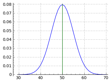
It seems that about 73% of the trial outcomes produce between 45 and 55 successes. Those familiar with the statistics of coin tosses may realize that by setting bounds like this we're sampling an underlying normal distribution that describes this class of outcome. Figure 2 shows a normal distribution (acquired with successive applications of the PMF function above), and below is a table, generated using the range form (a <= k <= b) above, that lists more sampling ranges and results:
Lower bound a Upper bound b Outcome 49 51 0.23564657 45 55 0.72874698 41 59 0.94311207 37 63 0.99336288 33 67 0.99959122 29 71 0.99998742 25 75 0.99999982 21 79 1.00000000
Figure 2 demonstrates that, as the number of trials increases, binomial probability outcomes converge on a normal distribution, and as the value of n increases, a binomial result becomes indistinguishable from a normal distribution. The real value of binomial probability lies with relatively small trial and success numbers, where discrete results are needed to properly characterize probabilities involving small numbers.
This special form of the CDF is the least often used, and it should not be applied to "equal to or greater than" problem statements. The reason? An "equal to or greater than" statement implicitly extends the probability sum range out to +∞, and my summation algorithm won't work very well if given an endpoint of +∞. Instead, to address "equal to or greater than" problem forms, use the prior cumulative distribution calculator to sum probabilities in the range (0 <= n <= k) and use the complement result, which will represent the sum of (k+1 <= n <= ∞).
This section shows the mathematical underpinnings of the above applications and examples.
First, the binomial distribution is discrete — it produces probabilities resulting from integer arguments, for example three oranges and five apples in a basket, as opposed to a fruit basket that, regardless of the number of elements, contains 62.5% apples. The latter kind of problem statement is more easily addressed using a normal distribution, which is by definition continuous.
Remember also about discrete binomial distributions that they resemble continuous normal distributions (see Figure 1 above), and in the limit of large values of n, the two distributions converge.
Factorial
Probability mathematics uses the factorial operation frequently, so we should start there. A factorial of x is indicated by $x!$, and it means:(1) factorial(x) = $ \displaystyle x! = \prod_{k=1}^{x} k = x \times (x-1) \times (x-2) ... $
Example: $5! = 5 \times 4 \times 3 \times 2 \times 1 = 120$
Note that the factorial function produces very large results for modest argument values. For example 170! = 7.25 x 10306, the largest factorial representable in a double-precision computer variable. This becomes important in a later discussion of algorithm design.
Combination
The combination function, variously rendered as "choose" or "choose(n,k)" or "nCk", describes how many unique sets of size k, in which order doesn't matter, can be drawn from a set of size n. It has this definition:
(2) choose(n,k) = $ \displaystyle {n \choose k} = \frac{n!}{k!(n-k)!}$
Note the special notation ${n \choose k}$ representing a combination. This shorthand notation is used in many binomial probability equations.
Permutation
The permutation function describes how many unique sets of size k, in which order does matter, can be drawn from a set of size n. It has this definition:
(3) permutation(n,k) = $ \displaystyle \frac{n!}{(n-k)!}$
Because the order of the elements matters in a a permutation, a permutation result will in general be larger than a combination result for the same arguments.
Probability Mass Function (PMF)
Apart from being useful in its own right, the PMF is the basis on which most other binomial probability functions are built. It has this definition:(4) pmf(k,n,p) = $ \displaystyle {n \choose k} p^k (1-p)^{n-k}$
The PMF tells us the probability of exactly k occurrences, each such occurrence having probability p, in a set of n Bernoulli trials, trials that are independent of each other and that produce one of two outcomes.
The PMF function can be described as multiplying the combination(n,k) result times the probability of k successes ($p^k$), times the complement of that probability (i.e. "failures") ($(1-p)^{n-k}$). The effect of these operations is to create a distribution of probabilities with respect to k that (a) is consistent with reality, and (b) resembles Figure 1 above.
Cumulative Distribution Function (CDF)

Remember that the same name is used for the binomial CDF and the normal distribution's CDF *, that they have certain properties in common, and that, as the value of n increases, their results converge. The binomial probability CDF has this form:
(5) cdf(k,n,p) = $ \displaystyle \sum_{i=0}^{\lfloor k \rfloor} {n \choose i} p^i (1-p)^{n-i}$
For contrast, here is the normal distribution version of the CDF:
(6) $ \displaystyle \Phi(x) = \frac{1}{\sqrt{2 \pi}} \int_{-\infty}^{x} e^{-\frac{t^2}{2}} dt$
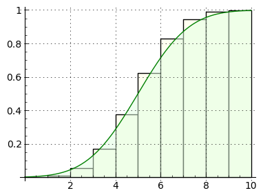
Note about these functions that the binomial version is discrete (it sums the results of integer arguments), while the normal distribution version is continuous (it accepts and integrates real arguments). In other respect the two functions are similar, because they address the same problem class in different ways. Figure 3 shows that they even look much alike when graphed.
In the world of pure mathematics, the presence of factorials and other similar functions serve only to identify the mathematical ideas as clearly as possible, and practical considerations have no standing. In applied mathematics by contrast, how we acquire results becomes important, and there are certain well-understood limitations in computer numerical processing.
Floating-point arithmetic
In practice and at the time of writing, most of the above calculations will be carried out using double-precision values whose properties are described in IEEE 754 (in this specification, a "double-precision" value is identified in the Basic Formats table as "binary64"). When working with double-precision (hereafter DP) values, several things become apparent:
Moving now to binomial probability calculations, one of the key problems is intermediate results. If we calculate a combination result for n = 200, k = 2, the result is a very reasonable 19,900. But the intermediate dividend is 7.88 x 10374, which exceeds the DP's exponent range and prevents the calculation from completing as expected.
Use of logarithms
Applied mathematics includes methods to squeeze more and better results from computer variables that have well-characterized limitations. In this case, an effective solution is to use logarithms — convert the values into logarithms, operate on them, and take the exponent of the result. To set the stage, here's an example that fails in the absence of special methods:
(7) combination(n,k) $ \displaystyle = \frac{n!}{k!(n-k)!}$
(8) combination(200,50) $ \displaystyle = \frac{7.88 \times 10^{374}}{3.04 \times 10^{64}(5.7 \times 10^{262})}$ $ \displaystyle = \frac{7.88 \times 10^{374}}{1.73 \times 10^{327}}$

That clearly won't work — both the dividend and divisor will overflow. To apply logarithms to a problem involving factorials, we need to use a special function named "log-gamma" ($\log\Gamma(x)$) that will require a bit of explanation.
Gamma and log-gamma
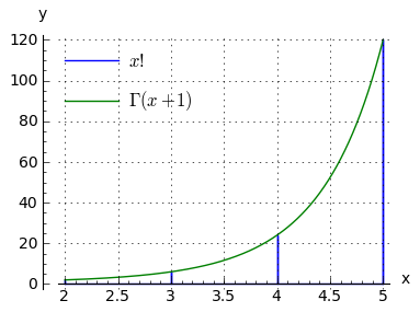
With respect to overflow issues, a factorial suffers from a number of problems, among which are that it's an integer — it would be more manageable if it could be made a floating-point value. The gamma function $\Gamma(x)$ does just that — it computes the factorials of both integers and non-integers, and places the results in the domain of the reals (Figure 4).
(9) $ \displaystyle x! = \Gamma(x+1)$
The gamma function places its result among the reals, but it won't solve the problem that the result will exceed the exponent range of a DP. A related function is designed for this specific purpose — the log-gamma function ($\log \Gamma(x)$), which simultaneously computes a factorial and takes its logarithm, placing the result in a reasonable numerical domain:
x x! $\log\Gamma(x+1)$ 1 1.00e+00 0.00 2 2.00e+00 0.69 4 2.40e+01 3.18 8 4.03e+04 10.60 16 2.09e+13 30.67 32 2.63e+35 81.56 64 1.27e+89 205.17 128 3.86e+215 496.41 256 inf 1167.26 512 inf 2686.06 1024 inf 6078.21 2048 inf 13571.95 4096 inf 29978.65 8192 inf 65630.83
For rows in which the scalar values have overflowed, the $\log\Gamma(x+1)$ values remain very reasonable.
Here's an example rendered in Sage, in which $\log\Gamma(x+1)$ makes an argument manageable:
sage: factorial(8192.0)
1.27588579940942e28503
sage: q = log_gamma(8193.0) ; q
65630.8265462913
sage: e^q
1.27588579941626e28503
sage: e^log_gamma(8193) - factorial(8192)
0
For those unaccustomed to reading scientific notation, 8192! ≅ 1.276 x 1028503. Click here to see 8192! expressed as an integer by Sage.
Also, take note — this applied mathematics activity of converting integers into floating-point values and processing them, normally produces approximate results, not exact. The resolution of the results often approaches the resolution of the floating-point values themselves, but obviously their accuracy is constrained by that same precision limit.
The rationale for using floating-point approximations is that, in most cases, uncertainties in data collection and preliminary assumptions are usually orders of magnitude greater than the errors produced by using floating-point values to process the results. A floating-point binomial probability result is typically accurate to ten or more decimal places, much more accurate than the assumptions and data that provide the computations's basis.
Here's a quick review of some rules for working with logarithms:
Normal operation Equivalent operation using
intermediate logarithms$y = a\ b$ $y = e^\left(\log(a) + \log(b)\right)$ $y = \frac{a}{b}$ $y = e^\left(\log(a) - \log(b)\right)$ $y = a^b$ $y = e^\left(\log(a)\ b\right)$
(Where $e$ = base of natural logarithms and $\log(x)$ = natural logarithm of $x$.)
Here is the classic PMF equation that, if carried out with normal computer variables, will fail for modestly large arguments:
(10) pmf(k,n,p) = $ \displaystyle \frac{n!}{k!(n-k)!} p^k (1-p)^{n-k}$
Applying the above rules, here is equation (10) using intermediate logarithms and the log-gamma function to prevent overflows:
(11) pmf(k,n,p) = $ \displaystyle \large e^{\log\Gamma(n+1) - \log\Gamma(k+1) - \log\Gamma(n-k+1) + \log(p) k + \log(1-p) (n-k)}$
The reason this works is because, although the PMF function's result is expressible within the numeric range of normal computer variables, without the use of logarithms the intermediate values will overflow before arriving at a result.
And that, boys and girls, is why the calculators on this page produce useful results with numerical arguments that virtually no other online calculators can handle.
Resources
As time passes, more languages and environments support the special functions described here and required for serious binomial probability work.
One or more Python libraries provide the essential binomial functions, implemented internally as explained above:
>>> from scipy.stats import *
>>> print( binom.pmf( 1000, 2000, .5 ) )
0.0178390111459
The Sage mathematical environment, where I do much of my development work and graph creation, includes log_gamma(x) and other primary binomial functions, either directly or by way of Python library imports as shown above.
For C++, there are public-domain resources online to add the essential functions to a project.
For JavaScript, this article's interactive elements include the essential functions, adapted from various online public domain sources including the above, optimized for the JavaScript environment and released under the GPL. As mentioned earlier, at the time of writing virtually no online binomial probability calculators are able to deal with anything more than small numerical values because they're written without benefit of logarithms.
| Home | | Mathematics | |  |  |  Share This Page Share This Page |